Multi-trip activity models

Introduction

Simple representations of transport systems based on origin-destination data often represent daily travel patterns as a single main trip per day, without distinguishing between multiple stages in a multi-stage trip (walk -> bus -> walk -> destination trips are simply represented as bus -> destination) or even multiple trips during the course of the day (omitting the fact that many people take a lunchtime trip to get lunch or simply to stretch their legs each day).

The concept of an ‘activity model’ aims to address these limitations by representing the complete list of activities undertaken by people throughout the day in the activity model. In this sense A/B Street can be seen as an activity model.

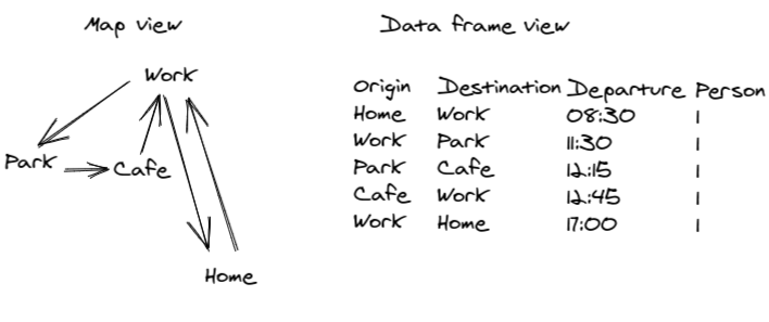
To show how A/B Street represents activity model data, we will take a hypothetical example, a trip from home to work and then to the park, to lunch and then to work before returning home after work. This 5 trip activity is more realistic that simple OD based models that just represents people travelling from home to work (and not back again in many cases), and is illustrated in the figure below.

How to get this information into a format for modelling? This article demonstrates how the data can be represented in R with the abstr package, and then converted into a format that can be imported by A/B Street.

library(abstr)

Minimal example

In R code, the minimal example shown above can be represented as two data frames (tabular datasets), one representing trip origins and destinations and the other representing movement between them, as follows:

places = tibble::tribble(
  ~name, ~x, ~y,
  "Home", -1.524, 53.819,
  "Work", -1.552, 53.807,
  "Park", -1.560, 53.812,
  "Cafe", -1.556, 53.802
)
places_sf = sf::st_as_sf(places, coords = c("x", "y"), crs = 4326)
plot(places_sf, pch = places$name)

# mapview::mapview(places_sf, pch = places$name)

od = tibble::tribble(
  ~o, ~d, ~mode, ~departure, ~person,
  "Home", "Work", "Bike", "08:30", 1,
  "Work", "Park", "Walk", "11:30", 1,
  "Park", "Cafe", "Walk", "12:15", 1,
  "Cafe", "Work", "Walk", "12:45", 1,
  "Work", "Home", "Bike", "17:00", 1
)

The two datasets can be joined, giving spatial attributes (origin and destination locations creating a straight line) for each OD pairs, using the od_to_sf() function from the od package as follows:

od_sf = od::od_to_sf(od, places_sf)
#> 0 origins with no match in zone ids
#> 0 destinations with no match in zone ids
#>  points not in od data removed.
plot(od_sf["departure"], reset = FALSE, key.pos = 1, lwd = 6:2)
plot(places_sf$geometry, pch = places$name, add = TRUE, cex =2)

# mapview::mapview(od_sf["departure"])

As an aside, another way of representing the spatial attributes of the OD data: four columns with ‘X’ and ‘Y’ coordinates for both origins and destinations:

(od::od_coordinates(od_sf))
#> Linking to GEOS 3.9.1, GDAL 3.4.0, PROJ 8.1.1; sf_use_s2() is TRUE
#>       ox     oy     dx     dy
#> 1 -1.524 53.819 -1.552 53.807
#> 2 -1.552 53.807 -1.560 53.812
#> 3 -1.560 53.812 -1.556 53.802
#> 4 -1.556 53.802 -1.552 53.807
#> 5 -1.552 53.807 -1.524 53.819

We will assign departure times and randomise the exact time (representing the fact that people rarely depart when they plan to, let alone exactly on the hour) with the ab_time_normal() function as follows:

departure_times = c(
  8.5,
  11.5,
  12.25,
  12.75,
  17
)
set.seed(42) # if you want deterministic results, set a seed.
od_sf$departure = ab_time_normal(hr = departure_times, sd = 0.15, n = length(departure_times))

The ab_json() function converts the ‘spatial data frame’ representation of activity patterns shown above into the ‘nested list’ format required by A/B Street as follows (with the first line converting only the first row and the second line converting all 5 OD pairs):

od_json1 = ab_json(od_sf[1, ], scenario_name = "activity")
od_json = ab_json(od_sf, scenario_name = "activity")

Finally, the list representation can be saved as a .json file as follows:

ab_save(od_json1, f = "scenario1.json")

Note: you may want to save the full output to a different location, e.g. to the directory where you have cloned the a-b-street/abstreet repo (see below for more on this and change the commented ~/orgs/a-b-street/abstreet text to the location where the repo is saved on your computer for easy import into A/B Street):

# Save in the current directory:
ab_save(od_json, f = "activity_leeds.json")
# Save in a directory where you cloned the abstreet repo for the simulation
# ab_save(od_json, f = "~/orgs/a-b-street/abstreet/activity_leeds.json")

That results in the following file (see activity_leeds.json in the package’s external data for the full dataset in JSON form):

file.edit("scenario1.json")

{
  "scenario_name": "activity",
  "people": [
    {
      "trips": [
        {
          "departure": 313400000,
          "origin": {
            "Position": {
              "longitude": -1.524,
              "latitude": 53.819
            }
          },
          "destination": {
            "Position": {
              "longitude": -1.552,
              "latitude": 53.807
            }
          },
          "mode": "Bike",
          "purpose": "Work"
        }
      ]
    }
  ]
}

You can check the ‘round trip’ conversion of this JSON representation back into the data frame representation as follows:

od_sf_roundtrip = ab_sf("activity_leeds.json")
# Or in the file saved in the abstr package
# od_sf_roundtrip = ab_sf(json = system.file("extdata/activity_leeds.json", package = "abstr"))
identical(od_sf$geometry, od_sf_roundtrip$geometry) 
#> [1] TRUE

Importing into A/B Street

Install the latest build of A/B Street for your platform.
Run the software, and choose “Sandbox” on the title screen.
Change the map to North Leeds. You can navigate by country and city, or search all maps.
Download data for Leeds, if this is your first time.
Change the scenario from the default “none” pattern, as shown below. Choose “import JSON scenario,” then select your scenario1.json file.

You should see something like this (see #76 for animated version of the image below):

Of course, the steps outlined above work for anywhere in the world. Possible next step to sharpen your A/B Street/R skills: try adding a small scenario for a city you know and explore scenarios of change.

Intermediate example: Sao Paulo

head(sao_paulo_activity_sf_2)
#> Simple feature collection with 6 features and 4 fields
#> Geometry type: LINESTRING
#> Dimension:     XY
#> Bounding box:  xmin: -46.64341 ymin: -23.56186 xmax: -46.63204 ymax: -23.54425
#> Geodetic CRS:  WGS 84
#> # A tibble: 6 × 5
#>   person      departure mode    purpose                                 geometry
#>   <chr>           <dbl> <chr>   <chr>                           <LINESTRING [°]>
#> 1 00240507101     30600 Transit Home       (-46.63204 -23.5592, -46.63422 -23.5…
#> 2 00240507101     33600 Walk    Shopping   (-46.63422 -23.55028, -46.64341 -23.…
#> 3 00240507101     63000 Transit Work       (-46.64341 -23.54499, -46.63204 -23.…
#> 4 00241455101     39600 Transit Home       (-46.63329 -23.56186, -46.63264 -23.…
#> 5 00241455101     45600 Transit Shopping   (-46.63264 -23.54425, -46.63508 -23.…
#> 6 00241455101     52200 Walk    Recreation (-46.63508 -23.55833, -46.63329 -23.…
sp_2_json = ab_json(sao_paulo_activity_sf_2, mode_column = "mode", scenario_name = "2-agents")

ab_save(sp_2_json, "activity_sp_2.json")

head(sao_paulo_activity_sf_20)
#> Simple feature collection with 6 features and 4 fields
#> Geometry type: LINESTRING
#> Dimension:     XY
#> Bounding box:  xmin: -46.63044 ymin: -23.55553 xmax: -46.629 ymax: -23.554
#> Geodetic CRS:  WGS 84
#> # A tibble: 6 × 5
#>   person      departure mode  purpose                                 geometry
#>   <chr>           <dbl> <chr> <chr>                           <LINESTRING [°]>
#> 1 00030710102     28800 Walk  Home    (-46.63041 -23.554, -46.63044 -23.55409)
#> 2 00030710102     46800 Walk  Work    (-46.63044 -23.55409, -46.63041 -23.554)
#> 3 00030710102     49200 Walk  Home    (-46.63041 -23.554, -46.63044 -23.55409)
#> 4 00030710102     61200 Walk  Work    (-46.63044 -23.55409, -46.63041 -23.554)
#> 5 00030743103     24900 Walk  Home    (-46.62906 -23.55553, -46.629 -23.55449)
#> 6 00030743103     25500 Walk  School  (-46.629 -23.55449, -46.62906 -23.55553)
sp_20_json = ab_json(sao_paulo_activity_sf_20, mode_column = "mode", scenario_name = "20-agents")

ab_save(sp_20_json, "activity_sp_20.json") # save in current folder, or:
# save to directory where you cloned the abstreet repo 
# (replace '~/orgs...' with the path to your local directory)
# ab_save(sp_20_json, "~/orgs/a-b-street/abstreet/activity_sp_20.json")

As with the Leeds example, you can import the data, after saving it with ab_save(). Use A/B Street to download São Paulo, then import the JSON file.

Robin Lovelace and Lucas Dias

Introduction

Minimal example

Importing into A/B Street

Intermediate example: Sao Paulo